1.5. Image quantization

Image quantization [1] describes the process of extracting meaningful information from images and converting them into discrete values which enable us to easily perform numerical computations.

Discrete images are often quantized by compressing a range of values into a single representative natural number, i.e.

\[f_h: \Omega_h \xrightarrow{ } \{0,...,N-1\}^m \quad \text{ with } \quad N\in \N.\]

The most common choices for the amount of different image values \(N\in\N\) are \(N=256\) or \(N=1024\).

Remark 1.2 (Processing quantized images)

In practice one would never perform numerical computations directly on the data structure of quantized images as large rounding errors would occur and lead to visible artefacts, e.g., color distortion or a loss of image quality.

To prevent these problems one typically uses the following processing pipeline:

1. Load a quantized image

2. Convert image values to float representation (e.g., IEEE 754 format)

3. Perform image processing on float values

4. Quantize resulting image again

5. Save quantized result

Definition 1.5 (Histogram)

Let \(\Theta:=\{z_j\in \R \mid j=1,...,N\}\) be a finite set of \(N\in \N\) real values.
Let \(a:=\min_{j=1,...,N}{z_j},b:=\max_{j=1,...,N}{z_j}\) be the minimal/maximal values in \(\Theta\).
We partition the interval \([a,b] \subset \R\) into \(m \in \N\) subintervals called bins, with fixed size \(h:=\frac{b-a}{m}\) via \(x_i=a + i\cdot h, \, i=0,...,m\).
These bins are labeled \(b_{i+1}=[x_i,x_{i+1}), \, i=0,...,m-2\) and \(b_m=[x_{m-1},x_m]\). The height of each bar and therefore the y-axis represents the number of datapoints in one bin, we call this frequency. With that, we define an (absolute) histogram \(H_{\Theta}: \{1,...,m\}\xrightarrow{ }\{0,...,N\}\) as

\[H_{\Theta}(k):=|\{z_j\in \Theta | z_j \in b_k\}|.\]

This function gives us the amount of data points in the k-th bin.

In this example there are two datapoints in the first bin, one datapoint in the second bin and so on. To put such histograms in a better perspective we scale the y-axis by \(\frac{1}{N}\). Then the height of one bar represent the percentage the total amount of data points in one bin.

Definition 1.6 (Relative Histograms)

The relative histogram \(h_{\Theta}: \{1,...,m\}\xrightarrow{ }[0,1]\) is defined as

\[h_{\Theta}(k) = \frac{H_{\Theta}}{N} \Rightarrow \sum_k h_\Theta = 1.\]

Thus \(h_\Theta\) is an estimator for a probability density function (PDF). In image processing such histograms find several important applications, for example Image quality assessment. A histogram gives a great overview of brightness, contrasts and the overall color range of the image as it plots the number of pixels of a certain shade over the value of said shade. Such histograms are called image histograms.

Definition 1.7 (Image histogram)

Let \(f_h:\Omega_h\xrightarrow{ }\{0,...,N\}\) be a discrete monochrome image. We define the (absolute) image histogram \(H_f:\{0,...,N-1\}\xrightarrow{ }\{0,...,\lvert \Omega_h \rvert\}\) as the amount of pixels with a certain gray value, i.e.,

\[H_{f_h}(k) \ \coloneqq \ \lvert \{ x \in \Omega_h:f(x)=k \} \rvert \quad \implies \quad \sum_{k=0}^{N-1} H_{f_h}(k)= \lvert \Omega_h \rvert.\]

The relative image histogram \(h_{f_h}:\{0,...,N\}\xrightarrow{ }[0,1]\) is defined as

\[h_{f_h}(k) = \frac{H_{f_h}(k)}{\lvert \Omega_h \rvert}.\]

A relative histogram is a discrete variant of a probability density function (PDF) as it encodes the probability that a random image pixel has a certain value.

Remark 1.3 (Coarse image histograms)

Sometimes one is not interested in the frequency of every possible image intensity value \(k \in \{0,\ldots,N-1\}\) of a discrete image \(f_h\), but rather in the amount of pixels that fall in certain value ranges, i.e., histogram bins with a width larger than \(1\).

In this case, we first specify the amount of resulting bins \(m \in \N^+\) and then regard a coarse image histogram with bin width \(\alpha \coloneqq \frac{N-1}{m}\) with frequencies:

\[H_{f_h}(k) \ \coloneqq \ | \{ x_i \in \Omega_h \, : \, f_h(x_i) \in [k \alpha, (k+1)\alpha) \}|.\]

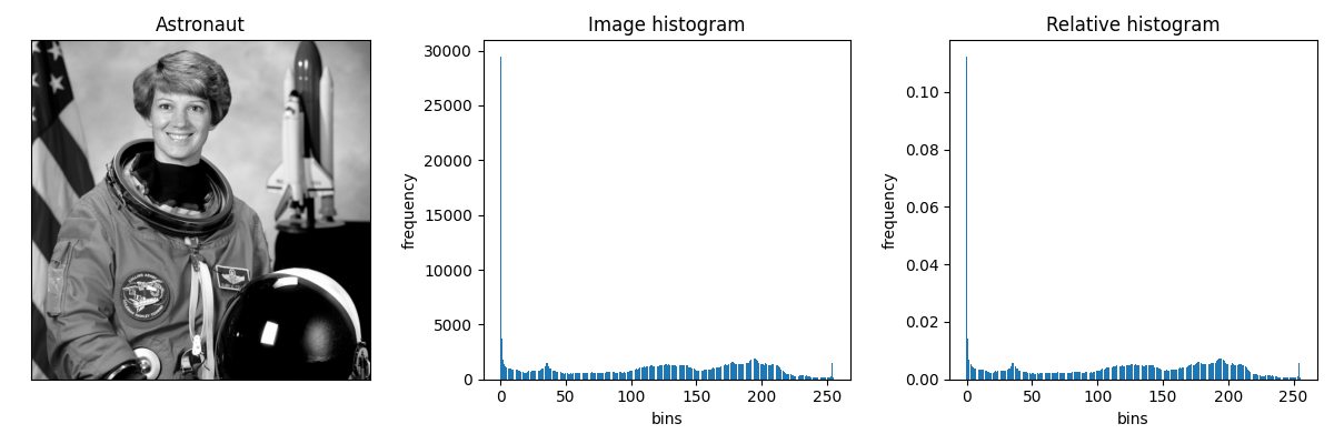
Fig. 1.1 Grayscale astronaut image with image histogram and relative histogram.

An image histogram yields a good graphical representation of a colors tonal distribution in one image. The x-axis represents the different shades of the color while the y-axis the number of pixel of each tonal value in the image. For an example see the following picture and the corresponding image histograms for red, green and blue tones.

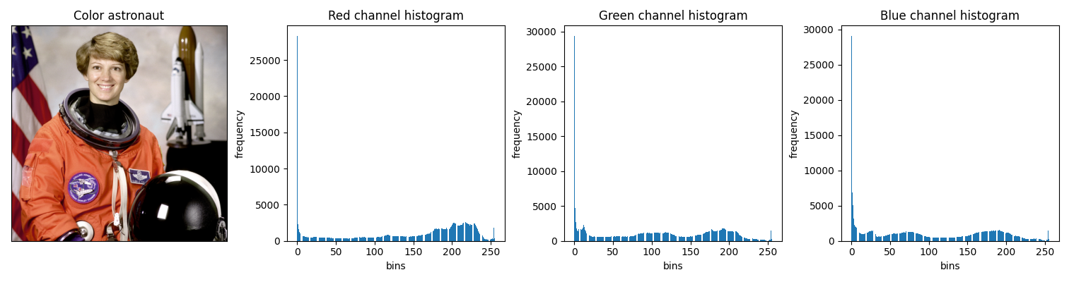
Fig. 1.2 Astronaut RGB image with histograms of the three color channels.

Important to understand is that the values further to the right of the x-axis represent higher and the values further to the left lower brightness. So the x-axis ranges from no brightness (pitch black) to maximum brightness (bright white).

The last piece of information to make working with image histograms easy as pie lies in so called cumulative image histograms.

Definition 1.8 (Cumulative image histogram)

We define a cumulative image histogram as

\[h_{c}(k) \ \coloneqq \ \sum_{i=0}^{k} h_{f_h}(i) .\]

This function is a discrete variant of a cumulative distribution function (CDF), which measures the probability that an image pixel takes a value less or equal than a specific number. Such a function gives information of how well contrasted an image is. The closer the Cumulative Image Histogram is to a line the better and wider contrasted the picture is. To change pictures based on their histogram we require a couple of tools.

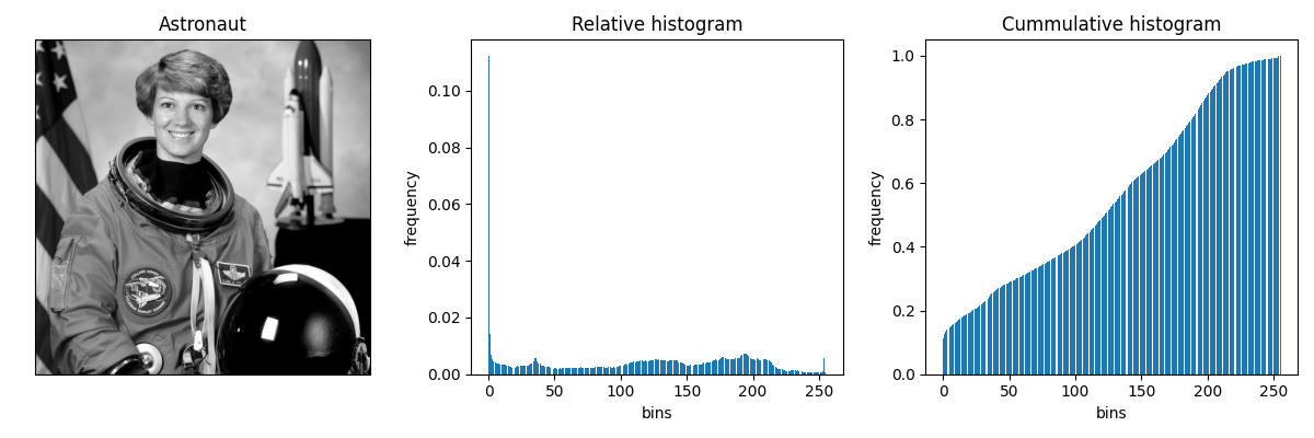
Fig. 1.3 Grayscale image of an astronaut with the respective relative and cumulative histogram.

---

[1]

In mathematics quantization is the process of mapping from continuous infinite values to a smaller, finite set of discrete values. An easy example would be to rank the taste of food with scores between 1 and 10.