2.2. Convolution

After discussing simple image transformations based on histogram manipulations before, we will introduce another family of methods that perform image filtering. The underlying concept of image filtering can simply be expressed by the mathematical convolution operator. In simple terms, a convolution is an operation combining the information of two functions to compute a new function. A convolution can be interpreted geometrically as sliding the first function over the second, while computing the overlapping area of both functions.

We begin by defining the continuous convolution operator in the following.

Definition 2.7 (Continuous convolution)

Let \(f,g \in L^1(\R^n; \C)\) be absolutely integrable functions. Then the convolution \((f*g) \in L^1(\R^n; \C)\) of the functions \(f\) and \(g\) is defined as:

\[(f*g)(x) \ \coloneqq \ \int_{\R^n}f(y)g(x-y)\,dy.\]

The convolution operator has some useful properties which we discuss in the following.

Remark 2.2 (Properties of convolution)

Let \(f, g, h\in L^1(\mathbb{R}^n;\C)\), then we have the following properties:

1. \(f*g=g*f\) (symmetry)

2. \(f*(g*h)=(f*g)*h\) (associativity)

3. \(f*(g+h)=f*g+f*h\) (distributive law)

4. \(\overline{f*g}=\overline{f}*\overline{g}\) (complex conjugation)

5. \((f*g)' = f'*g = f*g'\) (differentiation)

In the context of image processing the function \(f\) in the convolution is usually the image to be processed and the function \(g\) is a so called image filter. Depending on the particular choice of filter the convolution performs the task of smoothing, denoising, edge detection, etc.

There exists an interesting mathematical relation between the convolution and the Fourier transform.

Theorem 2.1 (Convolution theorem)

Let \(f, g\in L^1(\R^n;\C)\) be absolutely integrable functions. Then the following identity holds:

\[\mathcal{F}\left( f*g \right) \ = \ \mathcal{F} f \cdot \mathcal{F} g,\]

If \((\hat{f} \cdot \hat{g}) \in L^1(\R^n; \C)\) then by applying the inverse Fourier transform, we get:

\[\left( f*g \right) \ = \ \mathcal{F}^{-1} \left( \mathcal{F} f \cdot \mathcal{F} g \right).\]

For the sake of simplicity, we neglect here the normalisation factor \({(2\pi)}^{-\frac{n}{2}}\).

Proof. In the following proof we neglect the normalisation factor \({(2\pi)}^{-\frac{n}{2}}\) of the continuous Fourier transform to make following the proof easier.

\[\left(\mathcal{F}\left( f*g \right)\right) (\xi) \ = \ \int_{\mathbb{R}^n} (f*g)(x) e^{-i\langle \xi, x\rangle} dx \ = \ \int_{\R^n}\int_{\R^n}f(y)g(x-y)\,dy\, e^{-i\langle \xi, x\rangle}dx.\]

Introducing the auxiliary variable \(w := x-y\) yields \(x = w + y\), which does not change the integration limits as they are infinite. Thus, we get

\[\begin{aligned} &\int_{\R^n}\int_{\R^n}f(y)g(x-y)\,dy\, e^{-i\langle \xi, x\rangle}dx \ = \ \int_{\R^n}\int_{\R^n}f(y)g(w) e^{-i\langle \xi, (w+y)\rangle}\,dydw \\ = \ \quad & \int_{\R^n}\int_{\R^n}f(y)e^{-i\langle \xi, y\rangle} \cdot g(w) e^{-i\langle \xi, w\rangle}\,dydw \ = \ \int_{\R^n}f(y)e^{-i\langle \xi, y\rangle}\,dy \int_{\R^n}g(w)e^{-i\langle \xi, w\rangle}\,dw. \end{aligned}\]

Since the integration variables can simply be exchanged, we get

\[\begin{aligned} \int_{\R^n}f(y)e^{-i\langle \xi, y\rangle}\,dy \int_{\R^n}g(w)e^{-i\langle \xi, w\rangle}\,dw. \ &= \ \int_{\R^n}f(x)e^{-i\langle \xi, x\rangle}\,dx \int_{\R^n}g(x)e^{-i\langle \xi, x\rangle}\,dx. \\ & = \ \left(\mathcal{F}f\right)(\xi) \cdot \left( \mathcal{F}g \right)(\xi). \end{aligned}\]

This proofs the first identity of the convolution theorem.

Assuming that \((\hat{f} \cdot \hat{g}) \in L^1(\R^n; \C)\) we can simply prove the second identity by applying the inverse Fourier transform to the first equation:

\[\mathcal{F}^{-1} \left( \mathcal{F} f \cdot \mathcal{F} g \right) \ = \ \mathcal{F}^{-1}\left( \mathcal{F}\left( f*g \right)\right) \ = \ \left( f*g \right).\]

◻

To perform the convolution operation on discrete images we need a discrete analogue of the continuous convolution operator.

Definition 2.8 (1D Discrete convolution)

Let \(f_h,g_h:\Z\to \C\) be two discrete functions. The discrete convolution \((f_h * g_h)\) of \(f_h\) and \(g_h\) is defined as:

\[\left(f_h*g_h\right)_k \ \coloneqq \ \sum_{j=-\infty}^{+\infty}{{f_h}_j\cdot {g_h}_{(k-j)}}, \quad k\in\Z.\]

If the support of the two functions \(f_h\) and \(g_h\) is limited to a finite set of points \(\left[0, N-1 \right]\subset \Z\), then the discrete convolution simplifies to:

\[\left(f_h*g_h\right)_k \ = \ \sum_{j=0}^{N-1}{{f_h}_j\cdot {g_h}_{(j-k) \text{mod} N}}.\]

Because we are aiming to use the discrete convolution in the context of image processing the restriction to a finite set of points \(\left[0, N-1 \right)\subset \Z\) is meaningful.

Since the convolution is a linear operator (as follows from the distributivity property in Remark 2.2), the discrete convolution can be expressed as the following matrix-vector product:

\[(f_h*g_h) \ = \ \begin{pmatrix} g_0 & g_1 & &... & g_{N-1} \\ g_{N-1} & g_0 & & ... & g_{N-2} \\ \vdots & & & & \vdots \\ g_1 & ... & &g_{N-1} & g_0 \end{pmatrix}\begin{pmatrix} f_0\\ \vdots\\ \vdots\\ \vdots\\ f_{N-1} \end{pmatrix}=\begin{pmatrix} (f_h*g_h)_0\\ \vdots\\ \vdots\\ \vdots\\ (f_h*g_h)_{N-1} \end{pmatrix}.\]

The matrix has a particular structure as it periodically contains the discrete filter \(g_h\) shifted by one index per row. Indeed, we can easily show that this matrix-vector multiplication yields the discrete convolution \(\left(f*g\right)\). To demonstrate this let us regard the first entry \(\left(f_h*g_h\right)_1\) of the discrete convolution, which is given by

\[\begin{aligned} \left(f_h*g_h\right)_1 \quad &= \quad \sum_{j=0}^{N-1}{f_j\cdot g_{(j-1) \text{mod} N}} \\ &= \quad(f_0 \cdot g_{(1-0)\text{mod}N}) + (f_1 \cdot g_{(1-1)\text{mod}N}) + \dots + (f_{N-1} \cdot g_{(N-1)-1 \text{mod}N})\\ &= \quad (f_0 \cdot g_{(N-1)} + (f_1 \cdot g_0) + \dots + (f_{N-1} \cdot g_{(N-2)}) \\ &= \quad \begin{pmatrix} g_{(N-1)}, & g_0, & \cdots &, g_{(N-2)} \end{pmatrix} \cdot \begin{pmatrix} f_0, & f_1, & \cdots &, f_{(N-1)} \end{pmatrix}^T \end{aligned}\]

The following example computes the results of a one-dimensional discrete convolution via matrix-vector multiplication.

Example 2.1 (Convolution matrix)

Let \(g_h \coloneqq (0,\frac{1}{4},{\frac{\color{blue}1}2},\frac{1}{4},0)^T\) and \(f_h \coloneqq (0,1,1,1,0)^T\). Then we compute the discrete convolution via the following matrix-vector product:

\[g_h*f_h = \begin{pmatrix} 0& \frac{1}{4} & \frac{1}{2}& \frac{1}{4}&0 \\ 0&0 &\frac{1}{4} &\frac{1}{2} &\frac{1}{4} \\ \frac{1}{4}&0 &0 &\frac{1}{4} &\frac{1}{2} \\ \frac{1}{2}&\frac{1}{4} &0 &0 &\frac{1}{4} \\ \frac{1}{4}& \frac{1}{2}&\frac{1}{4} &0 &0 \\ \end{pmatrix} \cdot \begin{pmatrix} 0 \\ 1 \\ 1 \\ 1 \\ 0\\ \end{pmatrix} %\begin{pmatrix} % \frac{\color{blue}1}{\color{blue}2} & \frac{1}{4} & 0 & 0 & \frac{1}{4} \\ % \frac{1}{4} & \frac{\color{blue}1}{\color{blue}2} & \frac{1}{4} & 0 & 0 \\ % 0 & \frac{1}{4} & \frac{\color{blue}1}{\color{blue}2} & \frac{1}{4} & 0\\ % 0 & 0 & \frac{1}{4} & \frac{\color{blue}1}{\color{blue}2} & \frac{1}{4} \\ % \frac{1}{4} & 0 & 0 & \frac{1}{4} & \frac{\color{blue}1}{\color{blue}2} %\end{pmatrix} \begin{pmatrix} % 0 \\ % 1 \\ % 1 \\ % 1 \\ % 0\\ %\end{pmatrix} = \begin{pmatrix} 1\\ \frac{3}{4}\\ \frac{1}{4}\\ \frac{1}{4}\\ \frac{3}{4} \\ \end{pmatrix} = \begin{pmatrix} \left(f_h * g_h\right)_0 \\ \left(f_h * g_h\right)_1\\ \vdots \\ \vdots \\ \left(f_h * g_h\right)_{N-1} \end{pmatrix}\,.\]

.

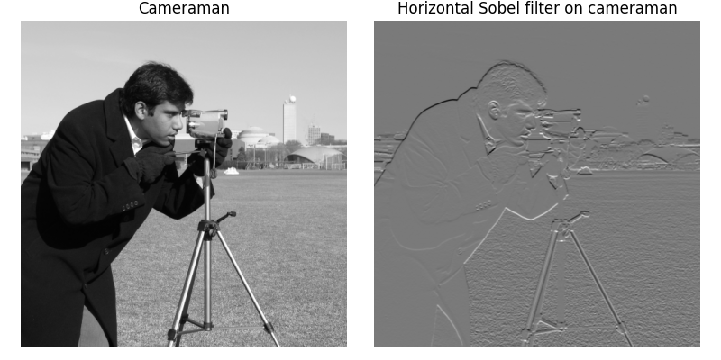
Fig. 2.2 Original grayscale image of the popular cameraman test image and convolution with the horizontal Sobel filter.

There exists also a discrete variant of the convolution theorem in Theorem 2.1, which we give in the following.

Theorem 2.2 (Discrete Convolution Theorem)

Let \(f,g: \Z^n\to \C\) be two discrete functions and at least one of them has compact support, i.e., it is zero outside a finite number of points. Then the following identity holds:\

\[\widehat{(f_h*g_h)} \ = \ N\cdot \hat{f}_h \cdot \hat{g}_h.\]

Proof. Exercise. ◻