2.1. Fourier transform

The Fourier transform is an important mathematical tool in signal processing and is popular in many different application tasks. Applying the Fourier transform to a suitable function allows one to decompose it into a continuous spectrum of frequencies.

Definition 2.4 (Continuous Fourier Transform)

Let \(f \in L^1(\R^n;\C)\) be an integrable function. Then the (continuous) Fourier transform \(\mathcal{F}:L^1(\R^n; \C)\to C_0(\R^n;\C)\) maps the function \(f : \R^n \rightarrow \mathbb{C}\) to its Fourier transform \(\hat{f}\) via:

\[\hat{f}(\xi) = (\mathcal{F}f)(\xi) \coloneqq {(2\pi)}^{-\frac{n}{2}}\int_{\R^n} f(x) e^{-i\langle \xi, x\rangle} \, \mathrm{d}x\,.\]

For the sake of notational brevity, we often denote the Fourier transform of \(f\) simply by \(\hat{f}\coloneqq \mathcal{F}(f)\).

The continuous Fourier transform is an invertible operator and the inverse Fourier transform \(\mathcal{F}^{-1}:L^1(\R^n; \C)\to C_0(\R^n;\C)\) of a function \(\hat{f} \in L^1(\R^n; \C)\) is defined as:

\[f(x) = (\mathcal{F}^{-1}\hat{f})(x) \coloneqq {(2\pi)}^{-\frac{n}{2}}\int_{\R^n} \hat{f}(\xi) e^{i\langle\xi ,x\rangle}d\xi.\]

We often denote the function we obtain by applying the inverse of the Fourier transform to \(\hat{f}\) as \(f\coloneqq \mathcal{F}^{-1}(\hat{f})\).

The Fourier transform has various interesting mathematical properties as we explain in the following.

Remark 2.1 (Properties of the Fourier transform)

1. The Fourier transform is (like many other operators, e.g. the gradient) a mapping between two function spaces, i.e., \(\mathcal{F}: L^1(\R^n; \C) \longrightarrow C_0(\R^n; \C)\), thus mapping an absolutely integrable function to a continuous function vanishing at infinity.

2. The Fourier transform is a linear mapping, i.e., it has the following property for all \(f,g \in L^1(\R^n; \C), \lambda, \mu \in \C\):

   \[\begin{split} \mathcal{F}(\lambda f + \mu g)(x) \ &= \ \lambda (\mathcal{F}f)(x) + \mu (\mathcal{F}g)(x) \\ \widehat{(\lambda f +\mu g)} \ &= \ \lambda\hat{f}+\mu\hat{g} \end{split}\]

3. One well-known function for \(n=1\) that is its own Fourier transform, i.e., \(\hat{f} = f\) is given by the Gaussian function

   \[f(x) = \frac{1}{\sqrt{2\pi}} e^{-0.5\lVert x \rVert^2}.\]

   This can be interpreted as a fixpoint of the Fourier transform \(\mathcal{F}(f) = f\) in \(C_0(\R^n; \C)\).

Since we are interested to apply the here discussed mathematical tools to digital images on a computer, we are interested in a notion of a discrete Fourier transform. This discrete Fourier transform does not transform a continuous function but rather a sequence of real or complex numbers.

We begin by defining the one-dimensional discrete Fourier transform in the following.

Definition 2.5 (1D Discrete Fourier Transform)

Let \(f_h=(f_0,...,f_{N-1})\in \mathbb{C}^n\) be a complex vector of samples of an underlying function f. Then the one-dimensional discrete Fourier transform (DFT) \(\hat{f}=(\hat{f}_0,...,\hat{f}_{N-1}) \in \mathbb{C}^n\) of \(f_h\) is defined as

(2.1)\[ \hat{f}_k \ = \ \sum_{j=0}^{N-1} f_j\cdot e^{-2\pi i \frac{jk}{N}} \quad k=0,...,N-1.\]

The inverse discrete Fourier transform (iDFT) \(f_h = \left(f_0,...,f_{N-1}\right)\in \mathbb{C}^n\) of \(\hat{f}_h\) is defined as:

\[f_k \ = \ \frac{1}{N}\sum_{j=0}^{N-1} \hat{f}_j e^{2\pi \frac{jk}{N}}.\]

The discete Fourier transform is periodic as we show in the following.

Lemma 2.1 (Periodicity of the DFT)

Let \(f_h=(f_0,...,f_{N-1})\in \mathbb{C}^n\) be a complex vector of samples of an underlying function \(f\). Then the one-dimensional discrete Fourier transform of \(f\) is N-periodic, i.e.,

\[\hat{f}_{k+N} \ = \ \hat{f}_k, \quad k=0,\ldots,N-1.\]

Proof. We prove the periodicity of the discrete Fourier transform directly by using the product rule for the exponential function:

\[\begin{aligned} \hat{f}_{k +N} \ &= \ \frac{1}{N}\sum_{j=0}^{N-1} f_j\cdot e^{-2\pi i \frac{j(k+N)}{N}} \\ &= \ \frac{1}{N}\sum_{j=0}^{N-1} f_j\cdot e^{-2\pi i \frac{jk+jN}{N}} \\ &= \ \frac{1}{N}\sum_{j=0}^{N-1} f_j\cdot e^{-2\pi i \frac{jk}{N}}\cdot \underbrace{e^{-2\pi i j}}_{=1}\\ &= \ \frac{1}{N}\sum_{j=0}^{N-1} f_j\cdot e^{-2\pi i \frac{jk}{N}} \ = \ \hat{f}_k. \end{aligned}\]

◻

In many cases, one has to apply the discrete Fourier transform to large amounts of data, e.g., to images with a high resolution. In these cases it makes sense to consider the asymptotic computational effort of the applied algorithm.

The computational complexity of the naive implementation of the one-dimensional discrete Fourier transform in (2.1) is \(\mathcal{O}(N^2)\) as one has to compute \(N\) multiplications and subsequent additions to compute one Fourier coefficient \(\hat{f}_k\) and this has to be performed for \(N\) coefficients for the complete discrete Fourier transform.

To improve the computational effort significantly one can exploit the famous fast Fourier transform.

Algorithm 2.1 (Fast Fourier Transform)

In the following we discuss the the one dimensional Fast Fourier Transform (FFT) in its simplest form proposed by [CT65]. This variant is also called the radix-2 decimation-in-time FFT.

Let \(f = (f_0,...,f_{2N-1})\in \R^{2N}\), \(f_{j}^{'} = f_{2j}\) and \(f_{j}^{''} = f_{2j+1}\). The \(k\)-th coefficient of the discrete Fourier transform \(\hat{f}_k\) is given in this case as:

\[\hat{f}_k \ = \ \frac{1}{2N}\sum_{j=0}^{2N-1} f_j \cdot e^{-2\pi i \frac{jk}{2N}}, \quad k=0, \ldots,(2N-1).\]

The fast Fourier transform of the k-th coefficient \(\tilde{f}_k\) can be efficiently computed by splitting the original vector \(f\) into two vectors of half length, i.e., the entries of \(f\) which are even- an odd-indexed, respectively:

\[\begin{aligned} \tilde{f}_k \ &= \ \frac{1}{2N}\left[\sum_{j=0}^{N-1} e^{-2 \pi i \frac{2j k}{2N}}\cdot f_{j}^{'} + \sum_{j=0}^{N-1} e^{-2 \pi i \frac{(2j+1)k}{2N}} \cdot f_{j}^{''}\right] \\ &= \ \frac{1}{2N}\left[\sum_{j=0}^{N-1} f_{j}^{'} e^{-2 \pi i\frac{jk}{N} } + e^{-2\pi i\frac{k}{N}} \sum_{j=0}^{N-1} f_{j}^{''} e^{-2 \pi i \frac{j k}{N}}\right] \\ &= \ \begin{cases} \hat{f}_{k}^{'} + e^{- \pi i \frac{k}{N}} \cdot \hat{f}_{k}^{''} & k < N \\ \hat{f}_{k-N}^{'} - e^{- \pi i \frac{k-N}{N}} \cdot \hat{f}_{k-N}^{''} & k\geq N. \end{cases} \end{aligned}\]

As \(k \geq N\) there exists an \(m\) with \(0\leq m < N\) and \(k = N +m\). This yields \(m= k - N\) and as \(\hat{f}\) is N-periodic: \(\hat{f}_m = \hat{f}_{m + N} \implies \hat{f}_{k-N} = \hat{f}_k\).

Based on the recursive nature of the above discussed Fast Fourier Transform it can efficiently compute a DFT of length \(N \in \N\) with a computational complexity of \(\mathcal{O}(N\log{N})\).

Since we typically process two-dimensional images, we require a two-dimensional variant of the discrete Fourier transform as well.

Definition 2.6 (2D Discrete Fourier Transform)

Let \(f \colon \Omega_h \rightarrow \C\) be a discrete \(M \times N\) image (with \(M\) rows and \(N\) columns), with data \(f_{k,l}\) for \(k=0,...,(M-1)\) and \(l=0,...,(N-1)\).

Then the two-dimensional discrete Fourier transform is defined as:

\[\begin{split} \hat{F}_{k,l} \ &= \ \frac{1}{MN} \sum_{m=0}^{M-1}\sum_{n=0}^{N-1} e^{-2 \pi i (\frac{mk}{M}+\frac{nl}{N}) } f_{m,n} \\ &= \ \frac{1}{M}\sum_{m=0}^{M-1}\left[\frac{1}{N} \sum_{n=0}^{N-1}e^{-2 \pi i \frac{n l}{N}} \cdot f_{m,n}\right] \cdot e^{-2 \pi i \frac{m l}{M}}. \end{split}\]

The two-dimensional inverse discrete Fourier transform is defined as:

\[f_{k,l} \ = \ \sum_{m=0}^{M-1}\sum_{n=0}^{N-1} e^{-2 \pi i (\frac{m \cdot k}{M}+\frac{n\cdot l}{N}) } \cdot \hat{F}_{m,n}.\]

While the naive implementation of the 2D discrete Fourier transform yields a computational complexity of \(\mathcal{O}(M^2N+N^2M)\) applying the Fast Fourier Transform from Algorithm 2.1 improves the efficiency up to \(\mathcal{O}(MN\log{MN})\).

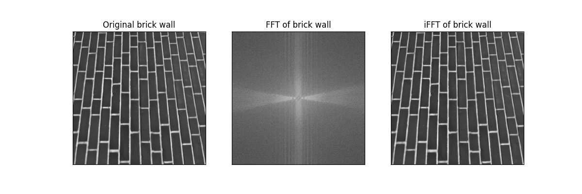
Fig. 2.1 Application of the 2D discrete Fourier transform and its inverse operation to a discrete image.