2. Image transformations

We can make use of image histograms in different ways. Using them we can perform simple image segmentation or image enhancement.

To achieve a better understanding of how to change a histogram and the affect it has on an image we must first take a look at so called linear transformation.

Definition 2.1 (Linear Transformation)

A linear transformation in context of image histogram performs a stretch/compression of the pixel intensity values from \([a,b]\) to \([l,L]\):

\[g(x) = \frac{f(x)-a}{b-a}\cdot(L-l)+l.\]

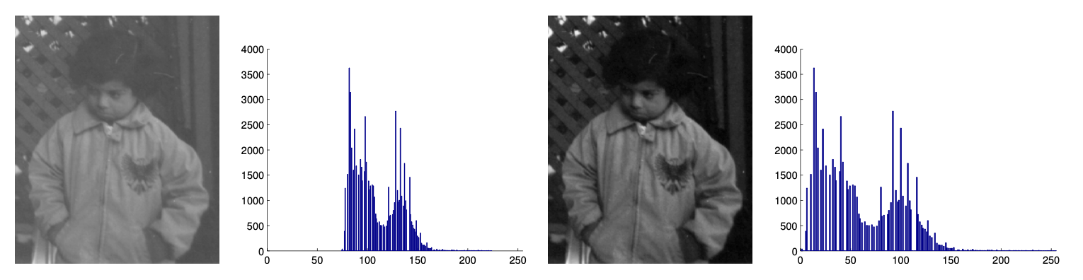
As one might see here we applied a linear transformation from the interval \([a,b] = [75,225]\) to \([l,L] = [0,250]\). The applied transformation would accordingly look like this:

\[\hat{H}_{\theta} = \frac{H_{\theta}-75}{225-75}\cdot(250-0) + 0\]

Where there is a linear transformation one might expect a non linear transformation. So we define the non-linear gamma transformation:

Definition 2.2 (Non-linear Gamma Transformation)

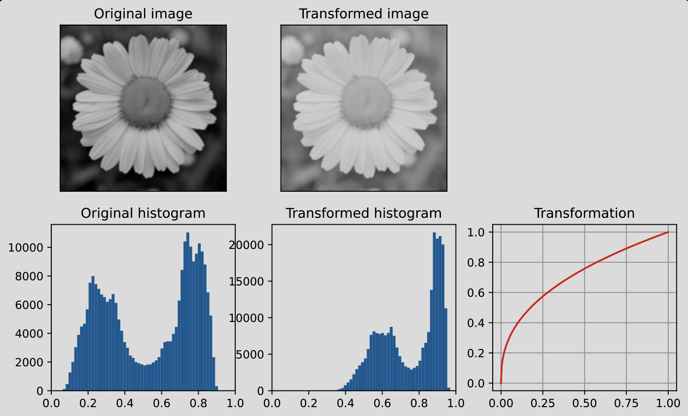
Contrary to the linear transformation which stretches or compresses more so the values on the x-axis, the gamma transformation, which is sometimes also called gamma correction, applies a stretch and compression along the y-axis according to the choice of the parameter \(\gamma\). The gamma transformation is defined as follows:

\[g(x)=255\cdot{\left(\frac{f(x)}{255}\right)}^\gamma \quad , \gamma>0.\]

In the following example we can see the impact of applying a gamma transformation with the choice of the parameter \(\gamma = 0.4\) has on the original image. While the pixel intensity values on the left side of the histogram get compressed into nothingness, the values stretch upwards more as we move further to the right.

The following graphic shows the different gamma functions.

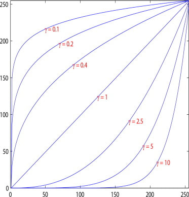
As one might imagine by the form of the gamma function one can estimate its impact it applies to a histogram. The higher our choice for \(\gamma\) is, the stronger the pixel intensity values on the far right get amplified while the values the further we move left get compressed/lowered. Choosing smaller a \(\gamma\) yields opposite results. As already mentioned nearing the cumulative distribution to a line the better the contrast of the image is. For this we have to equally distribute the pixel intensity values across the histogram. For this we require the following tool:

Definition 2.3 (Equalization)

For an image \(f\) of size \(M\times N\) pixels with gray-levels \(\{0,...,L-1\}\) the resulting function given by applying equalization to a histogram is defined as:

\[g_i = \lfloor (L-1) \sum_{k=0}^{f_i}h(k) \rfloor,\]

with \(h(k)=\frac{|\{i\in\Omega|f_i=k\}|}{MN}\)

The following graphic shows the effect of applying equalization.

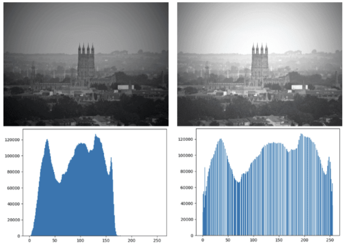
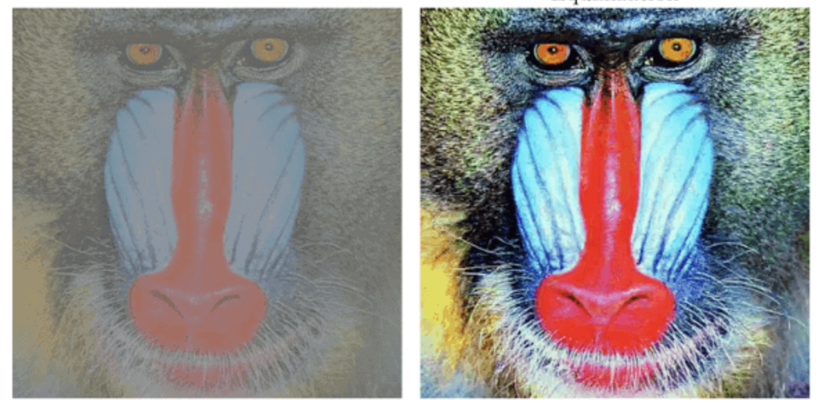
This example shows us exactly how the histogram changes and what effect it has on the image. Equalization spreads the pixel intensity values across the x-Axis without changing the individual values themselves. Simply put, we just change their location. Until now we only took monochrome images into account, though we can also apply our tools to colored images. Take an RGB image for example, to properly analyze it with histograms we would just need the histograms for red, green and blue shades. Applying equalization yields the following results:

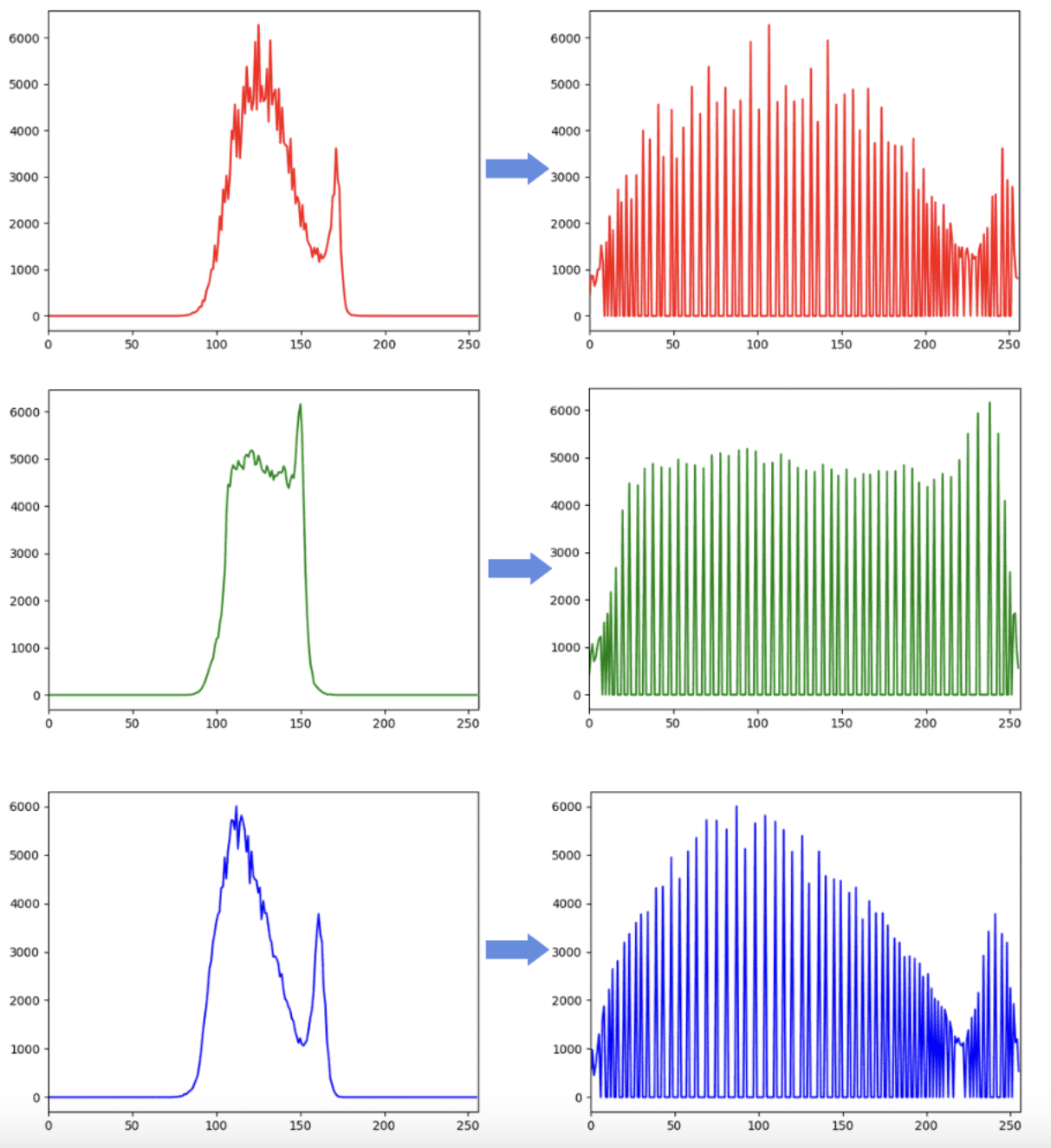
As we equalize the red, green and blue histogram we improve the contrast from the original image on the left to the equalized image on the right.